Example 2: Spectral calculations with CASTEP and run3
In this example, we will go from a crystal structure to a dispersion and DOS plot using run3, CASTEP and OptaDOS. For this use case, run3 uses the SeeK-path library to generate standardised band paths through reciprocal space to automatically compute a useful bandstructure for all crystal types.
Spectral calculations follow a similar setup to geometry optimisations: run3 expects to find a folder containing .res files with lattice/atomic position data, and one .cell and one .param file specifying the CASTEP options. Standard run3 rules apply: if a <seed>.res.lock file is found, or if the .res file is listed in jobs.txt, the structure will be skipped. Such a folder can be found in examples/bandstructure+dos/simple which contains some LiCoO2 polymorphs. The Jupyter
notebook simple_spectral.ipynb will also show you exactly how to run a standard BS/DOS calculation and plot the results with the API. The files in examples/bandstructure+dos/projected will show you how to use matador and OptaDOS to get projected densities of states and bandstructures. Here, we shall run through some more simple cases first.
run3 will follow some simple rules to decide what kind of spectral calculation you want to run. First, it will check the task and spectral_task keywords. The task keyword needs to be set to 'spectral' to trigger a spectral workflow. If spectral_task is either dos or bandstructure, then this calculation type will always be included in the workflow, with default parameters if unset. Otherwise, run3 will check the cell file for the
spectral_kpoints_mp_spacing (DOS) and spectral_kpoints_path_spacing (bandstructure) keywords and will perform either one or both of the corresponding calculation types. The first step will always be to perform an SCF calculation, which is continued from to obtain the DOS or BS (if any check file is found in the folder, run3 will attempt to skip the SCF and restart accordingly).
Both the bandstructure and DOS tasks can be post-processed with OptaDOS; run3 will perform this automatically if it finds a .odi file in alongside the .cell and .param. Similarly, if the write_orbitals_file keyword is set to True in the param file, orbitals2bands will be run automatically to reorder the eigenvalues in the .bands file. The output can be plotted using either the dispersion script bundled with matador, or through the API (see the Jupyter notebook).
Let us now consider some concrete examples.
Example 2.1: Bandstructure calculation with automatic path
We can compute just bandstructure by specifying spectral_kpoints_path_spacing and spectral_task = bandstructure in the cell and param respectively, e.g.
$ cat LiCoO2.param
task: spectral
spectral_task: bandstructure
xc_functional: LDA
cut_off_energy: 400 eV

$ cat LiCoO2.cell
kpoints_mp_spacing: 0.05
spectral_kpoints_path_spacing: 0.05
with .res file
$ cat LiCoO2-CollCode29225.res
TITL LiCoO2-CollCode29225
CELL 1.0  4.91 4.91 4.91 33.7 33.7 33.7
LATT -1
SFAC          Co Li O
Co        1       0.000000        0.000000        0.000000         1.000000
Li        2       0.500000        0.500000        0.500000         1.000000
O         3       0.255463        0.255463        0.255463         1.000000
O         3       0.744538        0.744538        0.744537         1.000000
END
Simply calling run3 LiCoO2 (with -v 4 if you want to see what’s going on) will perform three steps:
Analyse the lattice with SeeKPath, perhaps creating a primitive cell or standardising if need be, and generate the standard Brillouin zone path with desired spacing set by
spectral_kpoints_path_spacing.Perform a self-consistent singlepoint energy calculation to obtain the electron density on the k-point grid specified by
kpoints_mp_spacing.Interpolate the desired bandstructure path, yielding a
.bandsfile containing the bandstructure.
If you now run dispersion LiCoO2-CollCode29225 --png from the completed/ folder, you should see this:
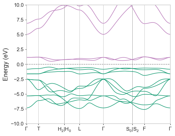
Note that the path labels are generated from the .cell/.res file in the completed/ folder, the .bands file does not contain enough information to make the entire plot portable. As mentioned above, if write_orbitals_file: true was found in the .param file, orbitals2bands would have been called to reorder the bands based on Kohn-Sham orbital overlaps.
Tip
Plots can be customised using a custom matplotlib stylesheet. By default, matador plots will use the stylesheet found in matador/config/matador.mplstyle, which can be copied elsewhere and specified by path in your .matadorrc under the plotting.default_style option. The default matplotlib styles can also be used directly by name, e.g. “dark_background”.
Tip
You can also specify a spectral_kpoint_path in your .cell file, that will be used for all structures in that
folder. This can be useful when comparing the electronic structure of e.g. defected cells. The dispersion
script will try to scrape the labels to use for plotting from the comments at the specification of the kpoint path,
e.g.
%block spectral_kpoint_path
0.0 0.0 0.0 ! \Gamma
0.5 0.0 0.0 ! X
%endblock spectral_kpoint_path
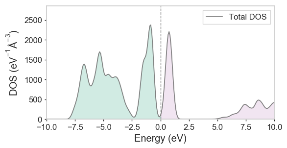
Example 2.2: A simple density of states (DOS) calculation
We shall now calculate the density of states in a similar way to the above, using the matador default for spectral_kpoints_mp_spacing, such that the cell file only contains kpoints_mp_spacing: 0.05 and the param file now has spectral_task: DOS.
Tip
If you are starting from the example above, you will need to move the .res file back into the current folder, delete the .txt files and rename the completed/ folder to e.g. completed_bs/. You might also consider moving the .check file to current folder, so that the calculation will re-use the SCF results.
Again, simply running run3 LiCoO2 will do the trick. Eventually, a .bands_dos file will be produced (any existing .bands files will be backed up and replaced at the end of the run). The dispersion script will recognise this as a density of states, and will apply some naive gaussian smearing that can be controlled with the -gw/--gaussian_width flag. Running dispersion LiCoO2-CollCode29225 --png -gw 0.01 will produce the following:
Tip
If you have a .bands file remaining in your top directory, dispersion will try to plot this as a bandstructure alongside your DOS, which may look terrible if .bands contains a DOS calculation! You can plot just the DOS using the --dos_only flag.
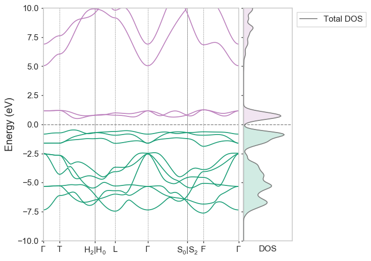
Example 2.3: Putting it all together
To run a DOS and bandstructure on the same structure, simply include both spectral_kpoints_mp_spacing and spectral_kpoints_path_spacing in your .cell file. Your spectral_task keyword in the param file will be ignored. This exact example can be found in examples/bandstructure+dos/simple, with an example Jupyter notebook showing how to make plots with the API directly, rather than the dispersion script.
After calling run3 again, the completed/ folder in this case should contain both a .bands and a .bands_dos file which can be plotted alongside one another using dispersion LiCoO2-CollCode29225, to produce the following:
Example 2.4: Using OptaDOS for post-processing: projected DOS and bandstructures
The final piece of the puzzle is OptaDOS, a package for broadening and projecting densities of states (amongst other things) that comes with CASTEP. By default, run3 will turn on the required CASTEP settings (namely pdos_calculate_weights) required by OptaDOS. In order for OptaDOS to be run automatically by run3, an extra .odi file must be added into our input deck, containing the details of the desired OptaDOS calculation.
Note
This example assumes that the OptaDOS binary is called optados and resides in your PATH, likewise orbitals2bands. This can altered by setting the run3.optados_executable setting in your matador config.
Warning
By default, OptaDOS will not be invoked with mpirun (i.e., your executable should work for serial runs too). A parallel OptaDOS run can be performed by setting the run3.optados_executable to e.g. ``mpirun optados.mpi`.
Warning
The projected dispersion curve feature is quite new to OptaDOS and thus is temperamental. Depending on when you are reading this, it may require you to have compiled OptaDOS from the development branch on GitHub.
run3 will try to perform three types of calculation: a simple DOS smearing, a projected density of states (with projectors specified by the pdos keyword), and a projected bandstructure (with projectors specified by the pdispersion keyword). If pdos/pdispersion is not found in the .odi, this corresponding task will be skipped. Likewise, if broadening is not found in the .odi, the standard DOS broadening will not be performed.:
$ cat LiCoO2.odi
pdos: species_ang
pdispersion: species
adaptive_smearing: 1
set_efermi_zero: True
dos_per_volume: True
broadening: adaptive
dos_spacing: 0.01
With all these files in place, simply running run3 LiCoO2 and dispersion (-interp 3 -scale 25) LiCoO2-CollCode29225 (optional flags in brackets) should yield the following plot:
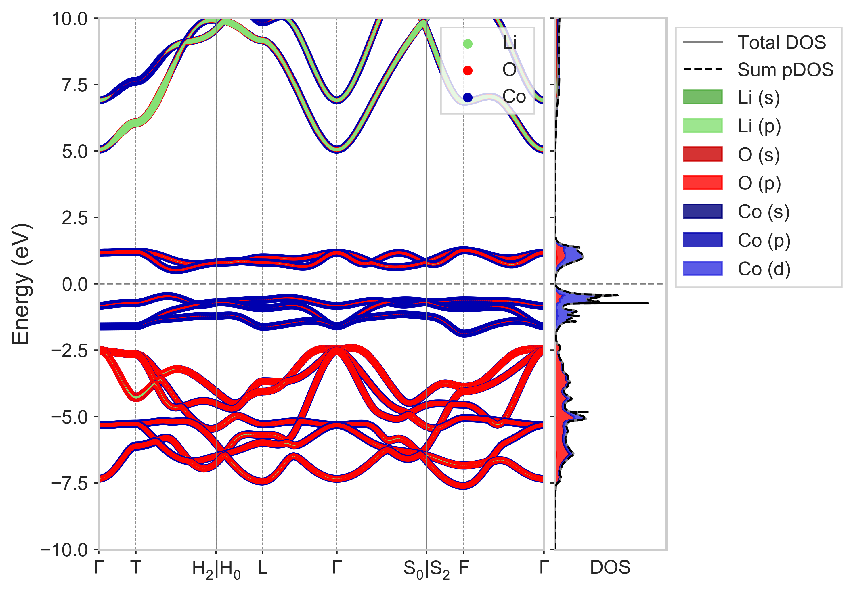
Tip
Note that the colours of each projectors in these plots is set by your VESTA colour scheme, which is bundled by default inside matador/config.